The MendelianRandomization R package provides a comprehensive set of methods for performing Mendelian randomization analyses with summarized data. We include methods for both single exposure (univariable) and multiple exposure (multivariable) analyses, as well as options to account for correlated variants in several methods.
Summarized data on genetic associations with traits and diseases from large consortia can be accessed using websites such as PhenoScanner and the GWAS catalog. These data can be used to obtain causal estimates following the Mendelian randomization paradigm. For an overview of this approach, see here for links to explanations and examples.
Installation
# Install released version from CRAN
install.packages("MendelianRandomization")
Usage
If you are just getting started with Mendelian randomization, we recommend following the brief example analysis below, and then working through the package component vignettes, starting with the data input vignette.
Bugs and Feedback
If you encounter any issues, bugs, or have suggestions for improvements for our R package, please report to the package maintainer Stephen Burgess.
We are keen to include further summarized data Mendelian randomization methods in our package, and any other customized code that you want to share with others. You can fork the package from Github to test for compatibility with the existing package.
Example analysis
This is an example analysis to investigate lipid effects on coronary artery disease risk using the example data included with the package.
library(MendelianRandomization) # load package

MRInputObject <- mr_input(bx = ldlc,
                          bxse = ldlcse,
                          by = chdlodds,
                          byse = chdloddsse)
The variables ldlc, hdlc, trig, and chdlodds are the genetic associations with (respectively) LDL-cholesterol, HDL-cholesterol, triglycerides, and coronary heart disease (CHD) risk for 28 genetic variants reported by Waterworth et al (2010). The respective standard errors of the associations are given as ldlcse, hdlcse, trigse, and chdloddsse.
Perform inverse-variance weighted method
We can use this package to perform a two-sample Mendelian Randomization analysis using a wide variety of methods. Here we show the inverse-weighted variance method:
MRAllObject_ivw <- mr_ivw(MRInputObject) # perform IVW method

MRAllObject_ivw  # view results
#>
#> Inverse-variance weighted method
#> (variants uncorrelated, random-effect model)
#>
#> Number of Variants : 28
#>
#> ------------------------------------------------------------------
#>  Method Estimate Std Error 95% CI       p-value
#>     IVW    2.834     0.530 1.796, 3.873   0.000
#> ------------------------------------------------------------------
#> Residual standard error =  1.920
#> Heterogeneity test statistic (Cochran's Q) = 99.5304 on 27 degrees of freedom, (p-value = 0.0000). I^2 = 72.9%.
#> F statistic = 28.0.

mr_plot(MRInputObject, line="ivw", interactive = FALSE) # plot results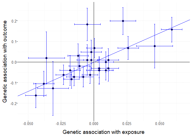
Alternative analysis methods
To assess the robustness of our results, we can perform other methods, such as the MR-Egger and weighted median methods:
MRAllObject <- mr_allmethods(MRInputObject, method="main") # perform MR-Egger and median methods

MRAllObject  # view results
#>           Method Estimate Std Error 95% CI        P-value
#>    Simple median    1.755     0.740   0.305 3.205   0.018
#>  Weighted median    2.683     0.419   1.862 3.504   0.000
#>              IVW    2.834     0.530   1.796 3.873   0.000
#>         MR-Egger    3.253     0.770   1.743 4.762   0.000
#>      (intercept)   -0.011     0.015  -0.041 0.018   0.451

mr_plot(MRAllObject) # plot results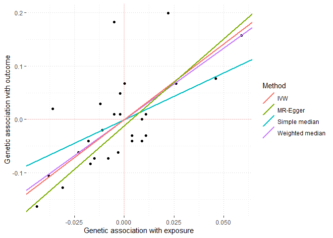
For more methods, see the vignettes on univariable and multivariable methods.